Archives for Mathematics

Continuation of my Calculus Journey

3rd June 2015 by artemlos under Mathematics, Posts

Introduction

During the two periods (from January), I’ve been working with with an interesting branch of mathematics – Multi Variable Calculus. Besides, I was studying Linear Algebra (see my other post) and Numerical Methods. Since I’m not actually supposed to study it in year 1, it was quite difficult when I needed knowledge of Linear Algebra to be able to understand certain concepts. In addition, there were clashes with other lectures and practice sessions, so I was effectively left with the course literature and other resources. This put me into a situation where I had to obtain the knowledge on my own and ensure that I understood the concepts. A friend of my (who took this course also) was sitting in the library and used other books that were available. My strategy was to use the original book in addition to the resources available online (such as other literature, videos, and Math SE). I think both strategies were really helpful in the study of Multi Variable Calculus. Here’s one thing I thought about two months after the course start:

$$ \displaystyle \underset{{Time\to \infty }}{\mathop{{\lim }}}\,Calculus=Physics$$

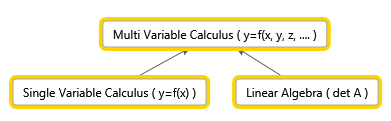
This is the connection between the subjects:

Spaces (3 to n space)

It’s quite convenient to translate real world problems into mathematical models, manipulate the data and interpret the result in a real world context. Since we live in a 3 dimensional world (at least, that’s the way many of us interpret it), many might already be familiar with $x,y,z$ coordinate system that allows us to express location of any object. But, if we were able to go from having things expressed in $2$d to $3$d, why not just go directly to $4$ or even $n$ space? Suddenly, we need to ensure that our definitions of concepts such as distance, neighborhood are clear and make sense even when we leave $3$ space.

Let’s look at neighborhood. If we simply think about a line with numbers, we could say that neighbors to a number $ p$ are numbers in the interval $(p-r,p+r)$. So, if we set $r=2$ and choose $p$ to be $3$, the interval is $(1,5)$. So, $1,2,4,5$ are some of the neighbors to $3$ at a distance $r$. Now, you might wonder why we look at the neighborhood. That’s simply to illustrate how things change when we add another dimension. Imagine that we are asked about the neighborhood to a point $p$ in $ 2$ space instead. Instead of a line, we get a disk with a radius $r$ centered at point $p$. In $3$ space, it’s a ball centered at $p$ of radius $ r$. The same trend will be observed when we started to look at the domain. For simple functions, the domain is a set of points on a line. For two variables, it is two-dimensional object and so on.

Cylindrical Coordinates

In single variable calculus, the polar coordinates might ring a bell. Cylindrical coordinates are quite similar. We basically perform the following substitution:

$$\left\{ \begin{gathered}
x = r\cos \theta \hfill \\
y = r\sin \theta \hfill \\
z = z \hfill \\
\end{gathered} \right.$$

The convention is that $r\ge 0$ and that $0 \le \theta \le 2\pi$. You might ask why we would need such coordinates? I had a similar question when I confronted them. They were more annoying than useful at the first sight (but spherical coordinates were even worse). However, once I started to deal with integrals with “strange” domains, they were a great relief. It will also be useful to know that the volume element is:

$$ \displaystyle dV=rdrd\theta dz$$

Spherical Coordinates

spherical

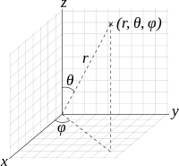
Spherical coordinates, as cylindrical coordinates, are based on a substitution that contains trigonometric functions. In this case, the substitution is:

$$ \displaystyle \left\{ \begin{array}{l}x=R\sin \phi \cos \theta \\y=R\sin \phi \sin \theta \\z=R\cos \phi \end{array} \right.$$

The convention is that $\displaystyle R\ge 0,\quad 0\le \phi \le \pi ,\quad 0\le \theta \le 2\pi $. The volume element that proves to be useful later is $\displaystyle dV={{R}^{2}}\sin \phi dRd\phi d\theta $.

Vector Functions

In many physics scenarios that appear in high school textbooks, problems are reduced two one/two dimensions. However, all of us know that the world has both a width, a breadth and a height. So, it can be useful to represent objects using three coordinates. If we disregard relativity for a moment, let’s say that the position of a particle is determined by time $t$. In other words,

$$ \displaystyle \left\{ \begin{array}{l}x=x(t),\quad y=y(t),\quad z=z(t)\\\vec{r}=(x(t),y(t),z(t))\end{array} \right.$$

So, you give me a time $t$ and I will be able to tell you where the particle is. In the same manner, we can express velocity and acceleration. That is,

$$ \displaystyle \vec{v}=\frac{d\vec{r}}{dt}=\left( \frac{dx}{dt},\frac{dy}{dt},\frac{dz}{dt} \right),\qquad \vec{a}=\frac{{{d}^{2}}\vec{r}}{d{{t}^{2}}}=\left( \frac{{{d}^{2}}x}{d{{t}^{2}}},\frac{{{d}^{2}}y}{d{{t}^{2}}},\frac{{{d}^{2}}z}{d{{t}^{2}}} \right)$$

Both velocity and acceleration have a magnitude and a direction, whereas speed has a magnitude only. However, in practice, we hear people use velocity and speed interchangeably. Anyway, given a velocity vector, it’s quite easy to find the speed, namely by taking the (euclidean) norm. That is,

$$ \displaystyle v=||\vec{v}||=\left\| \frac{d\vec{r}}{dt} \right\|={{\left( \frac{dx}{dt} \right)}^{2}}+{{\left( \frac{dy}{dt} \right)}^{2}}+{{\left( \frac{dz}{dt} \right)}^{2}}$$

Example: An object is moving to the right along the plane $y=x^2$ with constant speed $v=5$. Find $\vec v$ at $(1,1)$.

Solution: We simply need to express the movement in the plane as a vector, so since we $y=x^2, \quad \vec r =(x,x^2)$. By taking the derivative of $\vec r$, we get:

$$ \displaystyle \vec{v}=\frac{d\vec{r}}{dt}=\left( \frac{dx}{dt},2x\frac{dx}{dt} \right)=\frac{dx}{dt}(1,2x)$$

(do you recognize implicit differentiation? )We know that the speed is $5$, and that

$$ \displaystyle v=||\vec{v}||=\left| \frac{dx}{dt} \right|\sqrt{1+{{(2x)}^{2}}}=5$$

This implies that

$$ \displaystyle \frac{dx}{dt}=\frac{5}{\sqrt{1+{{(2x)}^{2}}}}=(\text{at point (1,1)})=\sqrt{5}$$

Therefore,

$$ \displaystyle \vec{v}=\frac{dx}{dt}(1,2x)=\sqrt{5}(1,2)$$

NB: Keep in mind that the $dx/dt$ term is not a vector, it’s a scalar.

Rules for Differentiation

They work in a similar way as in single variable calculus. There won’t be any nasty expressions, even if dot/cross product is involved. A word of warning: differentiation of vector functions only works if the basis vectors do not depend on the variable of differentiation. An example of the product rule with cross product: $\displaystyle \frac{d}{dt}(\vec{u}\times \vec{v})=\vec{u}’\vec{v}+\vec{u}\vec{v}’$.

Arc Length

After a minute of though, we quickly realize that the arc length is given by

$$ \displaystyle s=\int_{a}^{b}{\left| \frac{d\vec{r}}{dt} \right|dt=\int_{a}^{b}{|\vec{v}(t)|dt}}=\int_{a}^{b}{v(t)dt}$$

We might recall that when dealing with arc length of functions of one variable, the arc element (do you see the connection between the surface element?) happens to be $\displaystyle ds=\sqrt{1+{{\left( \frac{dy}{dx} \right)}^{2}}}dx$, which we can obtain by rearranging $\displaystyle {{(ds)}^{2}}={{(dx)}^{2}}+{{(dy)}^{2}}$ (Pythagoras’s theorem).

Functions of Several Variables

Before we move on to to 3 space, let’s look at one way we can get an understanding for 3 space using 2 space.

Level Curves

Suppose you are walking in a forest and have a map at your disposal. Even if the map is two dimensional, you are still able to apply it to the thee dimensional world. When you see a mountain, it is going to be expressed as a series of circles that indicate the “height”. The same can be done for functions of two variables. Say we have a paraboloid $\displaystyle {{z}}={{x}^{2}}+{{y}^{2}}$. To find the level curves, we replace $z$ with a constant $c$, i.e. $\displaystyle c={{x}^{2}}+{{y}^{2}}$. Now, this should be quite familiar to many, as it is the equation of a circle. By changing the $c$, we are actually changing the radius of the circle.

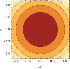
Contour plot

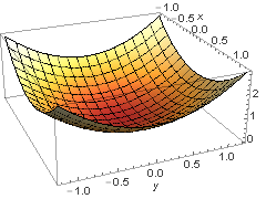
The 3d representation

It’s difficult to get a picture of the 4d world, but at least, using the same principle, it should be possible to gain an understanding.

Derivatives (Vector Calculus)

In Multi Variable Calculus, there isn’t just one operator that we can refer to as derivative. There are three of them:

grad – $\displaystyle \nabla f(x,y,z)=\left( {\frac{{\partial f}}{{\partial x}},\frac{{\partial f}}{{\partial y}},\frac{{\partial f}}{{\partial z}}} \right)\qquad \mathbb{R}\to {{\mathbb{R}}^{3}}$
div – $\displaystyle \nabla \cdot \vec{F}=\frac{{\partial f}}{{\partial x}}+\frac{{\partial f}}{{\partial y}}+\frac{{\partial f}}{{\partial z}}\qquad {{\mathbb{R}}^{3}}\to \mathbb{R}$
curl – $\displaystyle \nabla \times \vec{F}=\left( {\begin{array}{*{20}{c}} {\vec{i}} & {\vec{j}} & {\vec{k}} \\ {\frac{\partial }{{\partial x}}} & {\frac{\partial }{{\partial y}}} & {\frac{\partial }{{\partial z}}} \\ {{{F}_{1}}} & {{{F}_{2}}} & {{{F}_{3}}} \end{array}} \right)\qquad {{\mathbb{R}}^{3}}\to {{\mathbb{R}}^{3}}$

I think we might conclude that all of them use the same symbol (nabla). It’s quite interesting to point out that a lot of information is stored in the notation used. (ToK: Discuss the importance of conveying knowledge through notation)

Gradient

A gradient vector of a function is the normal vector of the function. The norm of a gradient vector tells the maximum rate of increase. The function at $(a,b)$ increases most rapidly in the direction of the gradient vector at point $(a,b)$.

Divergence

Divergence is a measure of the rate at which the field diverges, i.e. spreads away from a point $p$. I’ve observed that the net total flux of a solenoidal vector field ( $div \vec F =0$) is zero. This can be proved by a converting the flux integral into a triple integral using Divergence (Gauss) theorem.

Curl

Curl (rot in Swedish) is a measure of rotation, or differently phrased, how much a vector field swirls around a point.

Identities

Get ready, this will be a long list:

$$ \displaystyle \begin{array}{l}\nabla (\phi \psi )=\phi \nabla \psi +\psi \nabla \phi \\\nabla \cdot (\phi \vec{F})=(\nabla \phi )\cdot \vec{F}+\phi (\nabla \cdot \vec{F})\\\nabla \times (\phi \vec{F})=(\nabla \phi )\times \vec{F}+\phi (\nabla \times \vec{F})\\\nabla \cdot (\vec{F}\times \vec{G})=(\nabla \times \vec{F})\cdot \vec{G}-\vec{F}(\nabla \times \vec{G})\\\nabla \times (\vec{F}\times \vec{G})=(\nabla \cdot \vec{G})\vec{F}+(\vec{G}\cdot \nabla )\vec{F}-(\nabla \cdot \vec{F})\vec{G}-(\vec{F}\cdot \nabla )\vec{G}\\\nabla (\vec{F}\cdot \vec{G})=\vec{F}\times (\nabla \times \vec{G})+\vec{F}\times (\vec{G}\times \nabla )+(\nabla \cdot \vec{F})\vec{G}-(\vec{G}\cdot \nabla )\vec{F}\\\nabla \cdot (\nabla \times \vec{F})=\operatorname{div}curl\\\end{array}$$

Sometimes, it’s clear that they follow the same pattern as the usual product rule in single variable calculus. Some have to be derived brute force. Great that we don’t need to do it and instead can use them to build on top of this knowledge!

Directional Derivative

By looking at the gradient, we might have realized that a normal to surface is no longer a line (as is the case in single variable calculus), but rather a plane, or even a body of some sort. For functions with one variable, we only have one $\displaystyle \frac{dy}{dx}$, while the gradient contains three “derivatives”, $\displaystyle \left( \frac{\partial f}{\partial x},\frac{\partial f}{\partial y},\frac{\partial f}{\partial z} \right)$.

Now, back to directional derivatives. Really what it means is the rate of change of $f(x,y)$ at $(a,b)$ in the direction of a vector $\vec u$. It’s obtained by:

$$\displaystyle \frac{{\vec{u}}}{||u||}\nabla f(a,b)$$

The cool thing is that, in contrast to the gradient, the directional derivative actually gives us a value rather than a vector (set of values). Since the gradient points in the direction of the maximal increase, it can be useful to set it to be $\vec u$.

Keep in mind that $\vec u$ has to be a unit vector, otherwise, we will solve a different problem, namely, the rate of change of $f(x,y)$ at $(a,b)$ as measured by a moving observer (through $(a,b)$) with a velocity $\vec v$.

Taylor Polynomials

From single variable calculus, most of us will recognize Taylor series/polynomials. It’s a way to approximate functions close to a point by a polynomial. It’s quite similar to linearization where we could use the information we have about the slope and the function value in one point to predict the points in its neighborhood. By the way, in MVC, linearization formula looks like:

$$ \displaystyle f(x,y)\approx L(x,y)=f(a,b)+{{f}_{1}}(a,b)(x-a)+{{f}_{2}}(a,b)(y-b)$$

Since we don’t really have the concept of a tangent line, we have a tangent plane instead (the gradient is a set of derivatives, not just one). That’s why we have one $f$ with subscript 1 and another with subscript 2. Don’t get confused by my notation; the subscript indicates the index of the variable of integration, i.e. $\displaystyle {{f}_{1}}={{f}_{x}}$.

The general Taylor polynomial is given by

$$ \displaystyle f(\vec{a}+\vec{h})=\sum\limits_{{i=0}}^{m}{{\frac{{{{{(h\cdot \nabla )}}^{j}}f(\vec{a})}}{{j!}}}}+\frac{{{{{(h\cdot \nabla )}}^{{(m+1)}}}f(\vec{a}+\theta \vec{h})}}{{(m+1)!}}$$

or equivalently,

$$ \displaystyle f(\vec{a}+\vec{h})=f(\vec{a})+h\cdot \nabla f(\vec{a})+\frac{{{{{(h\cdot \nabla )}}^{2}}f(\vec{a})}}{{2!}}+\ldots +\frac{{{{{(h\cdot \nabla )}}^{m}}f(\vec{a})}}{{m!}}+\frac{{{{{(h\cdot \nabla )}}^{{m+1}}}f(\vec{a}+\theta \vec{h})}}{{(m+1)!}}$$

The questions I’ve been working with rarely required a polynomial of the third degree (if at all). Assuming that this will be the case during the exam, there’s a neat formula to remeber the the second order Taylor polynomial using a Hessian matrix (will describe under Extreme Value), namely,

$$ \displaystyle f(\vec{a}+\vec{h})=f(\vec{a})+h\cdot \nabla f(\vec{a})+\frac{1}{{2!}}{{\vec{h}}^{T}}\mathbf{H}\vec{h}$$

Exteme Values

Gradient(1st derivative test)

Gradient is a way to find the critical points of a function that occur at $\displaystyle \nabla g(x,y)=0$.

Hessian (2nd derivative test)

The Hessian matrix is a way to find whether a point is a maximum, minimum or a saddle point. There are four cases:

Positive definite -> local minimum
Negative definite -> local maximum
Indefinite -> saddle point
Other -> can’t tell.

Lagrange Multipliers

This might sound complex, but it’s all really about finding a maximum or minimum value of a function subjected to a constraint. There are two ways to think about it. In both ways, let $f(x,b)$ be a function subjected to the constrain $g(x,y)=0$. Then, we can work with a different function, that is, the Lagrange function: $\displaystyle L(x,y,z)=f(x,y)+\lambda g(x,y)$ and attempt to find its critical points. The way I think is better is to think about it though is by considering the fact that we want the gradient of the function to be parallel to the gradient of the constraint, i.e. $\displaystyle \nabla f(x,y)=\lambda \nabla g(x,y)$. Then, we simply need to solve the system of linear equations.

Integrals

In high school, many of us have been taught how to solve $$\int {f(x)dx} $$

Some of the techniques that might ring a bell are partial fractions, substitutions, etc. It might have been mentioned that integration is a way to find the area (depending on the definition) under the graph of a function $f(x)$. When I confronted MVC, I start to ask myself what each integral really represents, because it’s no longer possible to simply try to evaluate an integral.

Simple Integrals

By simple integrals, I mean $\displaystyle \iint\limits_{D}{{f(x,y)dA}}$ or $\displaystyle \iiint\limits_{D}{{f(x,y,z)dV}}$. Here’s an interesting thing that can be observed. $\displaystyle \int\limits_{D}{{dx}}$ is the length of the domain (a unit length), $\displaystyle \iint\limits_{D}{{dxdy}}$ represents the area of the domin (squared units), and finally $\displaystyle \iiint\limits_{D}{{dxdydz}}$ represents the volume of the domain (cube units). If we multiply by a function (inside the integral), we shift the definitions. Instead, the single integral will represent an area, the double integral will be a volume and the triple integral will be ….? Yeah, now we get into things that are quite hard to visualize. Basically, we would get a hyper volume.

Solving Simple Integrals

To solve simple integrals, we can, in most cases, use iteration. I’m not going to get into details, but basically, it’s a way to turn a double/triple integral into single integrals. However, at certain points, the domain we get might be very complicated. As an example, here’s a really simple iteration:

$$ \displaystyle \iint\limits_{\begin{smallmatrix}
0\le x\le 1 \\
0\le y\le 2
\end{smallmatrix}}{{xydxdy=\int\limits_{0}^{2}{{ydy\int\limits_{0}^{1}{{xdx=\{something\}}}}}}}$$

But, suppose we have a different case:

$$ \displaystyle \iint\limits_{{{{x}^{2}}+{{y}^{2}}\le 1}}{{{{x}^{2}}dxdy}}$$

This is not as obvious. However, we can perform a substitution (polar coordinates) to get $\displaystyle \iint\limits_{{{{x}^{2}}+{{y}^{2}}\le 1}}{{{{x}^{2}}dxdy}}=\int\limits_{0}^{{2\pi }}{{\int\limits_{0}^{1}{{{{r}^{2}}{{{\cos }}^{2}}\theta drd\theta }}}}$. Then, it’s quite easy to find the value. The important conclusion is that $\displaystyle dA=dxdy=rdrd\theta$. We can find the area/volume element by inserting into a Jacobian matrix, $\displaystyle \frac{{\partial (x,y)}}{{\partial (r,\theta )}}$.

Advanced Integrals?

The title is, to some extent, misleading, as the integrals aren’t that difficult but it might be harder to conceptualize them. All of the integrals I’m going to describe require understanding of vector fields, which will be described shortly below.

Fields and Integrals

This is the continuation of the previous section with focus on “advanced integrals”.

Fields

My understanding of fields is as a way to describe motion. We can, for instance, have a velocity field, which describes velocity at any given point. So, you give me a location and I will tell you the direction of the velocity vector at that point. In order to illustrate vector fields, we can try to find the field lines. Here’s how:

$$ \displaystyle \frac{{dx}}{{{{F}_{1}}(x,y,z)}}=\frac{{dy}}{{{{F}_{2}}(x,y,z)}}=\frac{{dz}}{{{{F}_{3}}(x,y,z)}}$$

The subscript, in this case, does not denote the partial derivative but rather the component of the vector field. By solving this differential equation, we are able to express the the field lines. For example, if the velocity field is $\displaystyle \vec{v}=(-y,x)$, we would get $\displaystyle \frac{{dx}}{{-y}}=\frac{{dy}}{x}\quad \Rightarrow \quad {{x}^{2}}+{{y}^{2}}=c$. Thus, the field lines will look like circles.

In addition, it’s important to keep in mind that there are both scalar fields and vector fields.

Physics and Fields

When I started to study this particular section, I thought it was great that I took physics higher level in high school. Concepts such as conservative fields, equipotential surfaces, etc., made more sense because of the prior knowledge. The cool thing about conservative fields occurs when we want to find the value of a line integral (described later). Since the definition of a conservative field that has the property $\displaystyle \vec{F}=\nabla \phi $, we can make an attempt to find the potential function $\phi$ instead and insert the desired starting and ending point. In conclusion, the conservative fields lead to path independence, i.e. it does not matter how we arrive at the end point.

Line Integrals

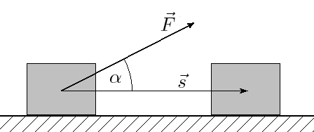
From (https://commons.wikimedia.org/wiki/File:Mehaaniline_t%C3%B6%C3%B6.png?uselang=ru)

Line integrals are pretty much based on the idea of finding the work (in physics). As we all know, work=force*distance. But, it’s only the x component we need, thus, $\displaystyle dW=|\vec{F}|\cos \theta ds$. This is the same as $\displaystyle dW=\vec{F}\cdot \hat{T}ds$. We know from single variable calculus that the tangent points in the direction of the derivative, so, $\displaystyle \hat{T}=\frac{{d\vec{r}}}{{ds}}$. Integrating this, we get: $\displaystyle \int\limits_{C}{{\vec{F}\cdot d\vec{r}}}$.

A good strategy is to parametrize the curve when evaluating a line integral.

Surface Integrals

Surface integrals are a step further than a line integral, analogous to the double integral that is a step further than a single integral.

$$ \displaystyle \iint\limits_{S}{fdS=}\iint\limits_{S}{f(\vec{r}(u,v))\left| \frac{\partial \vec{r}}{\partial u}\times \frac{\partial \vec{r}}{\partial u} \right|dudv=}\iint\limits_{S}{f(\vec{r}(u,v))\left| \frac{\partial (x,y,z)}{\partial (u,v)} \right|dudv}$$

As they are not quite the same as double integrals, we have to add a “term”, which can be though of as a conversion factor. In a double integral, we can think of the procedure as adding small rectangles and when we deal with surface integrals, we are essentially attempting the same thing, but a surface can be tilted and bent. So, we are projecting the it onto the $xy$ plane for instance. There’s going to be a slight difference between the area of the rectangle and the area of the surface, which we compensate using the conversion factor.

Flux Integrals

One of the parts of physics in high school that I found quite hard was flux. However, it’s not really that hard after a half a year of work! A flux integral is essentially a surface integral with some additional terms. Imagine we have a field and we put a surface of some kind in front of that field. If we put it perpendicular to the field (the normal of the surface will be parallel), everything will pass through. In contrast, if the surface is parallel to the surface (the normal vector is perpendicular), nothing will get through. We can relate to the dot product that exhibits similar properties $\displaystyle a\cdot b=0\quad \Leftrightarrow \quad a\bot b$. Below is a flux integral:

$$ \displaystyle \begin{array}{l}\iint\limits_{S}{\vec{F}\cdot \hat{N}dS=}\iint\limits_{S}{\vec{F}\cdot \left| \frac{\partial (x,y,z)}{\partial (u,v)} \right|dudv}\\\end{array}$$

Connecting Integrals

There are three important theorems in multi variable calculus that connect different kinds of integrals: Green’s theorem, Divergence theorem, and finally Stokes’s theorem.

Green’s Theorem (line = double)

If we have a closed curve, we are able to convert a line integral into a double integral and vice versa, i.e.

$$ \displaystyle \oint\limits_{C}{\vec F\cdot d\vec{r}=\iint\limits_{R}{\left( \frac{\partial {{{\vec{F}}}_{2}}}{\partial x}-\frac{\partial {{{\vec{F}}}_{1}}}{\partial y} \right)}}dA$$

Divergence (Gauss) Theorem (surface = tripple)

If we have a closed surface with a unit normal vector $\hat N$, we are able to go from a surface integral to a triple (simple) integral, and vice versa.

$$ \displaystyle \iiint\limits_{D}{div\vec{F}dV=\mathop{{\int\!\!\!\!\!\int}\mkern-21mu \bigcirc}\limits_C
\vec{F}\cdot \hat{N}dS }$$

Stokes’s Theorem (line = surface)

It’s a way to convert a line integral into a surface integral and vice versa.

$$ \displaystyle \oint\limits_{C}{\vec{F}\cdot d\vec{r}=\iint\limits_{R}{curl\vec{F}\cdot \hat{N}dS}}$$

Physics Applications (other applications)

Apart from those already mentioned, triple integrals can for instance be used to find the center of mass and the mass, i.e.

The x coordinate of the center of mas is given by $\frac{\iiint_D x dV}{\iiint_D dV}$
The density function $\rho$ can be integrated to get the mass $\iiint_D\rho(x,y,z) dV$

We might ask why we need functions of several variables. Well, the world has many relations where one value depends on several variables. For example, Finance. For example, Riksbanken probably has a mathematical model (I really hope!) of the way interest should be calculated, which can depend on both the interest in European counties, price of houses, etc. There are many variables, which will lead to situations where MVC knowledge will be useful.

Conclusion

I must say that each time I complete a course in mathematics, I get a new picture of the world. In the case of MVC, the great thing in my mind is the combination of single variable calculus and linear algebra (and of course, Physics). I guess it’s like philosophy, it makes you think in different ways.

Leave Comments →

The Beauty of Linear Algebra – Summary

12th March 2015 by artemlos under Mathematics, Posts, University

For almost a period I’ve had intense Linear Algebra (some days 4-6 hours), a subject that does not need that much prior learning to be able to understand. You need to know addition and multiplication, that’s it. Yet, the power of linear algebra in real world problems (and highly theoretical problems) is great. The aim of this post is to give a short overview of the subject, summarizing basic concepts.

Introduction

To translate problems into matrix equations can be quite useful. It can allows us to perform simple things as balancing chemical equations (use of Ax=b), take derivatives of polynomials, approximate solutions to overdetermined systems, rotate objects in any space, find volumes, interpret shapes, and so much more. If we think about the very basic concept – matrix multiplication – we simply follow certain rules (a definition) to find the answer. It is quite interesting that we can use this fact to “store” information in matrices, that is, a certain set of actions that have to be performed given a rule. An example of this is differentiation of polynomials (see the ToK marked with blue). Below, I’ve included some examples I constructed using MATLAB.

Euclidean Vector Spaces

Since this is simply a subset of General Vector Space and Inner Product Spaces, the interested reader is advised to read those sections instead.

General Vector Spaces

In this section we were introduced to the concept of vector spaces; basically generalizing euclidean vector spaces (3d). Below, some of the questions and focuses:

How do we find the shortest distance between two lines in n space? Answer, shortest distance is the perpendicular one (by Pythagoras thm). When I am concerned with such problems, I simply pick a general point on the lines, find the line that goes through these points (this expression will contain both $s$ and $t$), and use the power of calculus to find the shortest distance. Note, the calculus approach requires knowledge of multivariable calculus. Otherwise, remember that when dot product is zero, vectors are perpendicular (by definition).
What is a vector space? It might come as a surprise, but vector spaces are not only about vectors. We can have a polynomial vector space, matrix vector space, etc. The good thing here is that if we can prove that “something” is a vector space, then we are able to apply theorems for general vector spaces on these “something” vector spaces. We should prove that a) closed under addition ($\vec{u},\vec{v} \in V \implies (\vec{(u+v)}\in V)\ $), i.e. by adding vectors we never leave the vector space V, and b) that it is closed under scalar multiplication, ($\vec{v}\in V \implies k\vec{v}\in V, k \in \mathbb{R}$). A trick is to set the scalar to zero to show that something isn’t a vector space. Lastly, the beautiful thing about mathematics is that many times it’s all about definitions. If I want, I can come up with addition that behaves as multiplication, etc. It’s up to you to decide (we will later see in Inner product spaces that we can define the “dot” product also).
A subspace? As the name suggests, it’s a vector space that is inside another vector space. Same applies to these also; they should be closed under addition and scalar multiplication.
Linear dependent/independent? This is all about being able to express a vector as a linear combination of other vectors. If no vector in a vector space $V$ is expressible as a linear combination of other vectors in $V$, then these vectors are linearly independent. Ex. If a vector space is spanned by vectors $\{v_1,v_2,v_3\}$, then if we are unable to express these vectors in terms of each other, they are said to be linearly independent. Otherwise, they are linearly dependent. Recall cross product. We used it in “normal 3d space” (or more academically, orthonormal system with 3 basis vectors) to find a vector that is perpendicular to both vectors. NOTE: Linear independent vectors don’t need to be perpendicular, which is the case with cross product.
Basis? Above, we saw the use of basis without a proper definition. Not good. Basically, a basis is what makes up a vector space. It’s a set of vectors that are required to be a) linearly independent and b) they should span V (all vectors in V should be expressible as a linear combination of the basis vectors). To test if a basis is linearly independent, simply thrown them in into a matrix (in any direction), and evaluate the determinant. If it isn’t equal to zero, the vectors are said to be linearly independent.
Column space/row space/null space? Ok, we are getting into highly theoretical grounds (at least at this stage, it might seem so). Given $A$ is $m\times n$ matrix. Column space is the subspace of $\mathbb{R^m}$ that is spanned by the column vectors of $A$. The row space, as the name suggests, is the sub space of $\mathbb{R^n}$ that is spanned by the row vectors of $A$. The null space is the solution space (recurring definition) of $Ax=0$. A great theorem states that a system of linear equations $Ax=b$ is consistent if and only if $b$ is in the column space of $A$ ($b$ is expressible as a linear combination of column vectors of $A$). “The proof is similar to [..] and is left as an exercise to the reader“(book).
Theorems? Yes, it turns out that there is a formula that relates the dimension of the column space ($rank(A)$) and the dimension of the null space ($nullity(A)$). For a matrix with $n$ columns, we have that $ rank(A)+nullity(A)=n$. I would like to point out that dimension of the column space is equal to the dimension of the row space.
Orthogonal complements? A good relationship exists between the row space and the null space, and that is that they are orthogonal complements of each other. Orthogonal is a fancy way of saying perpendicular.
Is it possible to change basis vectors? Yes, this is perfectly fine. We use a matrix $T$ that will function as a converter (ToK: Discuss the importance of representing of a set of instructions in a more abstract form). Here’s the relationship, $$(\vec{v})_{B’}= {}_{B’}{T_B}(\vec{v})_{B})$$If we know the basis vectors of $B’$ and $B$, we can get the transition matrix by putting the basis vectors as columns in $[B’|B]$ and perform elementary row operations until we get to $[I|{}_{B’}{T_B}]$. In general, $$[new|old]\sim \text{el. row op.}\sim [I|old\to new]$$
How does the notion of functions apply to vector spaces? From high school, many of us should be familiar with the fact that a function maps one value to another value. This can be applied to vector spaces. Again, it’s always good to have a solid definition. We say that $T:V\to W$ is a function from vector space V to W, then T is a linear transformation if the following criteria is fulfilled: a) $T(k\vec{v})=kT(\vec{v})$ and b) $T(\vec{u}+\vec{v}) = T(\vec{u})+T(\vec{v})$. The good thing about being able to transform from one vector to another is that when this is put into a computer, we can do all sorts of cool things. For example, we can reflect, project, and rotate objects. We can also contract and dilate vectors, and this can be expressed in matrix form. Sometimes, we might want to perform two things at once, reflect and rotate maybe, then, we simply multiply the transformation matrices together in this order: rotate*reflect. Always think from right to left.

Inner Product Spaces

The fact that it is possible to generalize the notion of vector spaces suggests that the same can be done for operations that are performed inside a vector space.

What is an Inner product space (real vector space)? By definition, this is a vector space where we have an inner product with following properties.
1. $<\vec{u}|\vec{v}>=<\vec{v}|\vec{u}>$
2. $<\vec{u}|\lambda\vec{v}>=\lambda <\vec{u}|\vec{v}>$
3. $<\vec{u}|\vec{v} +\vec{w}>= <\vec{u}|\vec{v}> <\vec{u}|\vec{w}>$
4. $<\vec{u}|\vec{u}> \ge 0$ and $<\vec{u}|\vec{u}> = 0 \iff \vec{u}=0$
This is essentially the dot product in $\mathbb{R^n}$. The good thing about generalizing it is that “something” does not necessarily need to be in $\mathbb{R^n}$ to be an inner product space. For example, we can have an inner product space of all continuous functions (denoted by $C[a,b]$). Then, the inner product is defined as: $$<f(t)|g(t)>\int_a^b f(t)g(t)dt$$Since polynomials are continuous functions, this definition applies to polynomial inner product spaces.
What is perpendicularity (orthogonality)? In a a vector space with an inner product $ <\vec{u}|\vec{v}>$, the angle between $ \vec{u}$ and $ \vec{v}$ is defined as $$cos \theta = \frac{{ < \vec u|\vec v > }}{{||u||||v||}}$$Cauchy-Schwarz identity is quite useful and is given by: $<\vec{u}|\vec{v}>^2\le ||\vec{u}||^2||\vec{v}||^2$
How to project a vector on a subspace of an inner product space? Since we have a generalized version of the dot product, it’s possible to generalize the projection of a vector on a subspace. Here’s how: Given an orthogonal (this is crucial) basis for $W\in V$, say $\{ {{\vec v}_1} \ldots {{\vec v}_n}\} $ and that $\vec{u} \in V $, then: $${{\mathop{\rm Proj}\nolimits} _W}\vec u = \frac{{ < \vec u|{{\vec v}_1} > }}{{||{{\vec v}_1}|{|^2}}}{{\vec v}_1} + \ldots + \frac{{ < \vec u|{{\vec v}_n} > }}{{||{{\vec v}_n}|{|^2}}}{{\vec v}_n}$$
How to find an orthogonal basis? Note that the projection on “formula” only works if the basis is orthogonal. In order to find an orthogonal basis, we can use Gram-Schmidt process.$$\begin{array}{l}
{\rm{Step 1: }}{{\vec v}_1} = {{\vec u}_1}\\
{\rm{Step 2: }}{{\vec v}_2} = {{\vec u}_2} – \frac{{ < {{\vec u}_2}|{v_1} > }}{{||{{\vec v}_1}|{|^2}}}{{\vec v}_1}\\
{\rm{Step 3: }}{{\vec v}_3} = {u_3} – \frac{{ < {{\vec u}_3}|{{\vec v}_1} > }}{{||{{\vec v}_1}|{|^2}}}{{\vec v}_1} – \frac{{ < {{\vec u}_3}|{{\vec v}_2} > }}{{||{{\vec v}_2}||}}{{\vec v}_2}\\
\vdots \\
{\text{r times}}
\end{array}$$ Remember that $$ \vec u = {{\mathop{\rm Proj}\nolimits} _W}\vec u + {{\mathop{\rm Proj}\nolimits} _{{W^{\bot}}}}\vec{u}$$
How to find the “best” solution in an over-determined system? A good approach is to apply Least Square method. Over-determined systems occur in scientific measurements, and so if the error is assumed to be normally distributed, we can use the method of Least Squares. The idea is to think about the system’s column space and then try to project the measurements on the plane that the column space spans. It turns out that the best solution is $$x = {({A^T}A)^{ – 1}}{A^T}b$$ Keep in mind that it’s not required to have an orthogonal basis (i.e. the column space does not have to be orthogonal). Using this, we can express the projection formula as a simple matrix multiplication $${{\mathop{\rm Proj}\nolimits} _L}\vec u = A{({A^T}A)^{ – 1}}{A^T}b$$An interesting property that can be obtained is that $A^TA$ is invertible if and only if the column space of A is linearly independent.

Linear Transformations

I think the Swedish term linjär avbildning conveys more information rather than just stating linear transformation. The term basically means linear depiction, which is what this topic is about. At the first sight, this might seem as converting from one base to another. This isn’t entirely true, I’ve realized. It’s more appropriate to view this as a function that maps one value to another. As functions can be injective, surjective, bijective, it’s not implied that we should always be able to map a transformed point back to the original point. In contrast, when changing bases, it’s always possible to get from one basis to another; you never really introduce/remove more information.

How to define Linear Transformation? A linear transformation $A: V\to W$ should have the following properties:
1. $ A(\vec {u} + \vec {v}) = A(\vec {u}) + A(\vec {v}) $
2. $A(\lambda \vec u) = \lambda A(\vec u)$
What is Kernel and Image space(range)? If you’ve read what I wrote in General Vector Spaces, the Kernel = Null space and Image space = Column space.
Example? Let’s define the following linear transformation $$\begin{array}{l}
A(1,2,0) = (1,1,1)\\
A(0,1,2) = (0,1,1)\\
A(1,3,3) = (0,0,1)
\end{array}$$Unfortunately, this is not so useful if we want to transform a vector with the matrix A. It is easier if we would have the standard basis vectors on the left hand side. So, similar to the change in basis example, we put this into a matrix try to get an identity matrix on the left hand side. This method (Martin’s method) was discovered by Martin Wennerstein 2003. See the formal explanation of the method.
Relation between column space of composite linear transformations? Given that $B$ has full rank, i.e. $rank(B)=n$, then $rank(BA)=rank(A)$. Motivation: This is obvious if we consider the transformation $BA$ means. First, we perform transformation $A$, which will lead us to the image of A ($range(A)$). That is, all vectors will be depicted on the image space of $A$. When transformation $B$ is performed, all vectors in the image space of $A$ will be transformed using $B$. Note, $B$ kernel is trivial, i.e. the zero vector transforms to zero vector.
What’s special about the kernel? It can be useful to think of kernel as “the information that gets lost during a transformation”(KTH student). For example, if the kernel contains more than just a zero vector (i.e. it’s non-trivial), when we perform a transformation, some vectors will be depicted on the zero vector; thus “information” disappears.
What is injectivite, surjective, and bijective? Let $A:V \to W$. Injective (one-to-one) is if $\vec x \ne \vec x’ \implies A(\vec x) \ne A(\vec x’)$, i.e. each vector is represented by a unique vector (so we can map back to the original vector after a transformation). Surjective (onto) is if $\forall \vec y \in W\exists \vec x \in V:\vec y = A\vec x$, i.e. for all vectors in the image of $A$, we can map it to the original vector. Bijective is when it’s both injective and surjective.
Properties? For something to be injective, the dimension of the kernel has to be zero. For $A: V\to W$ to be surjective, $dim ker(A)=dim(W)$. This can be proved by the dimension theorem and the definition of surjectivity.

Eigenvalues

An eigenvalue is the value lambda in $A\vec x = \lambda \vec x$. It can be, for instance, applied in problems such as a) Find $$ {A^{1000}}\left( \begin{array}{l}
2\\
1
\end{array} \right) $$given that we know A, or b) express $2x_1^2+ 2x_2^2+2x_3^2+4x_1x_2$ (see this) without the cross product terms. The latter is particularly good when identifying shapes that have been rotated/transformed.

How to find eigenvalues? Simply solve $ \det (A – \lambda I) = 0$, the characteristic equation.
How to find the eigenvectors corresponding to eigenvalues? Solve $(A – \lambda I)\vec x = 0$.
Express a matrix using eigenvalues and eigenvectors? We can always express a matrix A as $A = PD{P^{ – 1}}$. If P happens to be orthogonal (i.e. the rows/columns space forms an orthonormal base), then we can express it as $ A = PD{P^T}$ because of a property of orthogonal matrices that states that $A{A^T} = I$ or equivalently that $ {A^{ – 1}} = {A^T}$.
Raising matrices to a certain power? It can be shown that ${A^k} = P{D^k}{P^{ – 1}}$.
Applying orthogonal deagonalization on quadratic form? $$\begin{array}{l}
a{x^2} + b{y^2} + c{z^2} + d{x_1}{x_2} + e{x_1}{x_3} + f{x_2}{x_3} = \\
= ({x_1},{x_2},{x_3})\left( {\begin{array}{*{20}{c}}
a&{d/2}&{e/2}\\
{d/2}&b&{f/2}\\
{e/2}&{f/2}&c
\end{array}} \right)\left( \begin{array}{l}
{x_1}\\
{x_2}\\
{x_3}
\end{array} \right)
\end{array}$$Now, this can be seen as $x^TAx$. If we make a substitution $\vec x = P\vec y$ such that $P$ orthogonaly diagonalizes $A$, then $$ {x^T}Ax = {(P\vec y)^T}A(P\vec y) = {y^T}({P^T}AP)y$$
Orthogonal matrices? In an orthogonal matrix, the row vectors form an orthonormal base (same for column vectors). An interesting property that exists when multiplying a vector $x$ is $$||A\vec x||=||\vec x||$$ and $$A\vec x * A \vec y=\vec x* \vec y$$Then, as we mentioned previously, the inverse of an orthogonal matrix is simply the transpose (please see my answer for a possible application).

CodeProject

Leave Comments →

A book for young computer scientist

30th December 2014 by artemlos under Education, Mathematics, Posts, University

Today, I published one of my summer projects – a book (a chapter) – as open-source, on GitHub. The reason why it’s open source, the purpose and goal, and finally how I got started is described below.

Why open source?

The initial aim of the book was to make computer science mathematics more accessible, which shaped it quite a lot. First of all, the programming language used is JavaScript, which I believe is the one many people have access to. Not all languages are like that, and some you have to pay for. JavaScript, on the other hand, can be access on all machines (computers, phones) that have access to a web browser. Secondly, the book can, from now on, be accessed free of charge. The code (written in TeX) is also available. I hope that this will allow an even greater audience able to access it. Thirdly, each chapter (right now it’s only one) should describe the subject from scratch. It’s not assumed that you should have some prior knowledge to be able to understand it.

Purpose and goal

I’ve partly described it above, but there is more to it. There are two groups the book should target: young programmers and non-programmers. Regarding the first group, my experience tells me that there is a tendency that many young programmers skip the underlying concepts of mathematics behind some computer operations and instead focus on the code (in some cases, you don’t even need to code that much). The latter group will still find many concepts interesting and my goal is to show that computer science is fun and not as scary as they might think.

How it started

The first time I came across this idea is when I was contacted by an editor at Apress in the beginning of November 2013. Before that, I recently published a short course reference for Algorithms via C# course, which I haven’t had the opportunity to start properly (see KSDN). After a consultation with one of my teachers, I decided to keep focused on the diploma to get good grades and later on the book. So, sometime in June I started writing the chapter about modular arithmetic that I thought I knew a lot of about. But, when I started writing I had to continue doing research and learn the concepts (from several sources) and later write it down. Since I want to write it in my own phase (when I have time) and want people to have access to it, it’s not published as a traditional book but rather as a digital one.

More information

Leave Comments →

“Trits” instead of “bits” – a short introduction to balanced ternary

20th December 2014 by artemlos under Mathematics, Posts, University

It’s usually said that students who would like to study computer science should familiarize themselves with binary representation of numbers and thus get used to very common powers of 2, i.e. 2¹=2, 2²=4, 2³=8, etc. That’s definitely true; the digital world we live in uses bits and almost all programming languages are based on Boolean algebra. But, just because something is popular does not mean it’s good. In this short article, my aim is to give the reader a general understanding of the concept of balanced ternary, the benefits of using it, and finally some history of earlier attempts to create ternary computers.

Intro

The concept Balanced ternary has many underlying ideas, so let’s try to break it down into things we can relate to. The word ternary, in this context, refers to ternary numeral system. A numeral system is a way different people express numbers: the Great Greeks used a superscript on letters to identify numbers, i.e. α’, β’, γ’. In the Roman Empire, they used I, II, III, IV (we still use these numbers in names, i.e. Charles XII). Many people nowadays use numbers like 0, 1, 2, 3, 4, 5, 6, 7, 8, 9 (origin from Hindu-Arabic numbers). This way of writing numbers can be referred to as base 10 or simply decimal. A ternary numeral base is similar to decimal, but allows only 0, 1, 2. In binary (base 2), we only allow 0, 1.

Decimal (Base 10)	0	1	2	3	4	5	6	7	8	9	10
Ternary (Base 3)	0	1	2	10	11	12	20	21	22	100	101

A clear observation from this table is that once digits end (i.e. going from 9 to 10), we put a zero and carry a 1 forward (in the number). This is similar to base 3, however, since we only have 0, 1, 2, our digits end faster than in base 10.

There exists an algorithm to convert between different bases, but that would probably be better suited for another article. Therefore, it’s not going to be discussed here (convert numbers). However, it’s quite simple to convert from base 3 to base 10 by an interesting observation. For example, 123 is equivalent to saying that 123= 1*10²+2*10¹+3*10⁰ = 1*100+2*10+3. In base 3, we have a similar approach, but instead of 10, we use 3. Say we want to convert 22 (in base 3) to base 10. Therefore, 2*3¹+2*3⁰=2*3+2=8 (in base 10). This conclusion goes hand in hand with the one in the table.

Now, we should have some grasp of ternary numeral systems. Let’s move on to the term balanced. A intuitive way of thinking about it that something should be balanced, like masses on opposite sides of a weight should cancel out. So, how would such system look like? I turns out that instead of saying that we can use digits 0, 1, 2 we instead introduce -1 so that the digits in the balanced ternary system are -1, 0, 1 (looks to be balanced?). Let’s refer to the -1 as n and 1 as p. The table below links the numbers in base 10 with the ones in balanced ternary.

Decimal (Base 10)	0	1	2	3	4	5	6	7	8	9	10
Balanced Ternary (Base 3)	0	p	pn	p0	pp	pnn	pn0	pnp	p0n	p00	p0p

There is a similar pattern here as for unbalanced ternary. The interested reader should consider to experiment with this concept by implementing it in the favourite programming language (see all implementations).

Benefits

Here are some of the benefits of the balanced ternary:

The sign (+/-) is stored in the number, and can be deduced by the leading trit (similar to bit). So, if a number starts with -1, or using our notation, n, we know it’s negative.
In order to get the number with the opposite sign, simply replace all n‘s with p‘s and all p‘s with n‘s. Eg. Since 7 is pnp, -7 is npn.
In order to round to the nearest integer, the fractional part should be removed.
Things don’t have to be either true or false. There exists an unknown case also.

History

It might seem that this idea works in theory but not in real computers. However, this is not true. At Moscow State University, a series of Setun computers was developed. The first Setun was built in 1958. An interesting thing that can be noted is that it used ternary logic.

Further reading

For those who are interested, please take a look at the links below:

Edits:

Corrected the base10-base3 table.
First published 20.12.2014 (dd/mm/yyyy)

CodeProject

Leave Comments →

The Power of Finite Differences in Real World Problems

19th October 2014 by artemlos under C#, Mathematics, Posts

Introduction

Most of the people are certainly familiar with Calculus already from high school and the beginning of university. It is usually associated with concepts like infinitely small, behaviour at infinity, finding the area under the graph, and finding the rate of change. It seems to be so much about infinity (which is difficult to imagine) but not that much about finite values. So why not look at finite differences instead? In this article, we are going to see how powerful the concept difference is, and how we can apply it to real world problems. First, we are going to look at how the difference can be found in a sequence. Secondly, the way we can find the next term and later on how we can get a formula to generate the nth term. Finally, we are going to use the idea of finding the nth term to find an expression of the sum.

The difference operation

It is quite intuitive, once we see a sequence, to try to find the difference between adjacent terms. If we are not satisfied, we look at the difference of the differences, and so on. Our aim now is to construct a method that will behave like we normally would in this situation. First, however, let’s look at what happens when we take the difference of each term.

$a_0$
	$a_1-a_0$
$a_1$		$a_2-2a_1+a_0$
	$ a_2-a_1$		$a_3-3a_2+3a_1-a_0$
$a_2$		$a_3-2a_2+a_1$
	$a_3-a_2$
$a_3$

We can take the difference as many times as we like, but given that a sequence was constructed with only addition, subtraction, multiplication and division i.e. it was a polynomial, there is going to be a point when we can stop taking the difference. The important thing now to realize from this figure is that the difference expression contains the coefficients from the Pascal’s triangle. This is good if we want to take the difference many number of times. The code below utilizes this observation.

/// <summary>
/// Finds the difference between terms in a sequence. By chaging the degree, we can take difference of the differences.
/// </summary>
/// <param name="sequence">The sequence of doubles passed in as a double array.</param>
/// <param name="term">The index of the first term where the diff. should be taken. NB: As the degree increases, the smaller can the term be</param>
/// <param name="degree">The type of difference, i.e. if degree=1, the first difference is taken and if degree=2, the difference of the first difference is taken. </param>
/// <example>If the sequence is {1,2,3,4,...}, term=0, degree=1, we get 1. By changning degree=2, we get 0.</example>
/// <returns>The difference between the terms in the sequence, depending on the degree.</returns>
public static double GetDifference(double[] sequence, int term, int degree)
{
    // the pascal's triangle should be optimized. we only need half of the values

    double result = 0;

    bool evenStart = (term + degree) % 2 == 0 ? true : false;

    int j = 0;

    for (int i = term + degree; j <= degree; i--)
    {
        result += Pascal(degree, j) * sequence[i] * (evenStart ? (i % 2 == 0 ? 1 : -1) : (i % 2 == 0 ? -1 : 1));
        j++;
    }

    return result;

}

Finding the next term

Before we proceed in finding the next term and ultimately the polynomial describing the nth term, let’s focus our attention on a real world example. Say we have the sequence $\{n^2\}$ i.e. $1, 4, 9, 16 \dots$. We assume that we don’t know the nth term, i.e. we only know some values of the sequence. The common procedure in this case is to look at the differences, similar to the previous section. For example,

$1$
	$3$
$4$		$2$
	$ 5$		$0$
$9$		$2$
	$7$
$16$

To be sure that we’ve found a pattern, we should end up at zero (assuming a polynomial generated the sequence). The interesting thing about this figure is that we know that each difference in the table can be expressed in terms of the difference expressions in the previous section. So, $3=(4)-(1)$ and $2 = (9)-2\times (4)+(1)$. This idea hints us to a possible way of finding the next term in the sequence. Since we know that the second difference $2$ is constant, we can find an expression for the next term by some simple arithmetic. That is, $2=a_n -2\times a_{n-1} + a_{n-2}$. Thus we can find the nth term given the two terms before it. This is done by the following code:

/// <summary>
/// Finds the next term in the sequence, given that a pattern exist.
/// </summary>
/// <param name="sequence">The sequence of doubles passed in as a double array.</param>
/// <param name="term">If term=-1, the next term in the sequence is going to be found. By default, you don't need to change this variable.</param>
/// <returns></returns>
public static double GetNextTerm(double[] sequence, int term = -1)
{
    int constantIndex = 0;

    if (HasPattern(sequence, out constantIndex))
    {
        double constant = GetDifference(sequence, 0, constantIndex - 1);

        if (term == -1)
        {
            // have find the term to start with to figure out the n+1 term.
            term = sequence.Length - constantIndex; 
        }

        double result = 0;

        bool evenStart = (term + constantIndex - 1) % 2 == 0 ? true : false;

        int j = 1;

        result += constant;

        for (int i = term + constantIndex - 1; j <= constantIndex - 1; i--)
        {
            result += Pascal(constantIndex - 1, j) * sequence[i] * (evenStart ? (i % 2 == 0 ? 1 : -1) : (i % 2 == 0 ? -1 : 1));
            j++;
        }

        return result;
    }

    throw new Exception("The sequence does not contain a recognized pattern.");
}

Finding the expression for the nth term

This is a bit more tricky to find in contrast to what we’ve done so far. The nth term is very dependent on the number of times the difference operation has to be taken before we end up at zero. In the previous example, we had to take it three times to get to zero. The polynomial we got had the second degree. It turns out that if we had to take the difference $n$ times to get to zero, the polynomial is of the degree $n-1$. This is quite useful, because if we know how the polynomial looks like, the only thing we need to find are the coefficients (more in-depth tutorial).

In the sequence $1,4,9,16\dots$, we had to take the difference three times, so the polynomial has the second degree, i.e. $ax^2+bx+c$. We have three unknowns, so we need three data points to solve the system of equations. That is,

$\left[ {\begin{array}{*{20}{c}} 1 & 1 & 1 & 1 \\ 4 & 2 & 1 & 4 \\ 9 & 3 & 1 & 9 \end{array}} \right]$

When we reduce this matrix to echelon form, we get that the coefficient for $n^2 $ is $1$, and zero for the remaining terms. The code below does this task.

/// <summary>
/// Finds the coefficients of the nth term and returns them in a double array.  The first item in the array is of the highest power. The last term in the array is the constant term.
/// </summary>
/// <param name="sequence">The sequence of doubles passed in as a double array.</param>
/// <param name="degree">The degree value returned here is the number of times we have to take the differnce of this sequence (using GetDifference) to get the difference to be zero.</param>
/// <returns></returns>
public static double[] GetCoefficientsForNthTerm(double[] sequence, int degree)
{
    var mat = new Matrix(degree, degree + 1);

    for (int i = 0; i < degree; i++)
    {
        for (int j = 0; j <= degree; j++)
        {
            if (j == degree)
            {
                mat[i, j] = sequence[i];
            }
            else
            {
                mat[i, j] = Get.IntPower(i + 1, (short)(degree - j - 1));
            }

        }
    }

    mat.RREF();

    var output  = new double[degree];

    for (int i = 0; i <  degree ; i++)
    {
        output[i] = mat[i, degree];
    }

    return output;
    
}

The coefficients we get correspond to a term in the polynomial. For example, if we get $3, 2, 1$, the polynomial is $3x^2+2x+1$.

Finding the closed form for the sum

When we first think about how we can find the closed form for a sum, we might conclude that it is difficult. In Concrete Mathematics – A Foundation for Computer Science, an entire chapter (chp. 2) and a great part of other chapters is dedicated to sums, and the way we can find the anti-difference. At least, that was my thought when I got this idea. But later, an interesting thought came up to my mind, and that is to treat the sum as a sequence and the sequence as the difference of the sums’ terms. Let’s clarify this. If we have the sequence $ 1,2,3,4,\dots$, we can construct the partial sums, i.e. $1, 1+2, 1+3+4, 1+2+3+4$, thus $1, 3, 6, 10$. But the partial sums form a new sequence which we can analyse in a similar way. This means that can we can reuse quite a lot of code. Now, since in the original sequence $ 1,2,3,4,\dots$, we have to take the difference twice to get zero, in the new sequence $1, 3, 6, 10$, we have to take the difference three times. The code for doing this is shorter, in contrast to the previous ones.

/// <summary>
/// Finds the coefficients of the closed form of the sum and returns them in a double array. The first item in the array is of the highest power. The last term in the array is the constant term.
/// </summary>
/// <param name="sequence">The sequence of doubles passed in as a double array.</param>
/// <param name="degree">The degree value returned here is the number of times we have to take the differnce of this sequence (using GetDifference) to get the difference to be zero.</param>
/// <returns></returns>
public static double[] GetCoefficientsForNthSum(double[] sequence, int degree)
{
    double[] partialSums = new double[sequence.Length];

    partialSums[0] = sequence[0];
    for (int i = 1; i < sequence.Length; i++)
    {
        partialSums[i] = partialSums[i - 1] + sequence[i];
    }

    return GetCoefficientsForNthTerm(partialSums, degree + 1);
}

Limitations

One of the limitations of this code/algorithm is that we can only use sequences that have been generated by a polynomial. Exponents are not allowed, although $n^2= n\times n$, so that works. The reason is quite simple. Formally, we define difference as an operator on a function (similar to derivatives) as

$\Delta f(x) = f(x+1) – f(x)$. Let’s say we have $f(x)=2^x$. If we take $\Delta(2^x)=2^{x+1}-2^x=2^x(2-1)=2^x$. Not good, no matter how many times we take the difference, we end up with the same thing we had in the beginning. This is why this particular algorithm does not work in this case. It is possible to add an extra step that checks against known sequences each time a difference is taken. This, I will do a bit later! 🙂

Source code

You can find all additional methods in the FiniteCalculus class in Mathos.Calculus (Mathos Core Library). Also, you can see this code in action here!

CodeProject

Leave Comments →

Application of knowledge about number bases in problems

30th September 2014 by artemlos under Mathematics, Posts

During the 2 hours journey to Stockholm from Bjursås, I found an interesting way of illustrating solutions to problems with a certain pattern. In this case, it was a recursion problem. The problem is as following (From Concrete Mathematics – A Foundation for Computer Science 2nd edition):

Problem

Solve the recurrence:

Eqn1

Assume that

Solution

When we look at several cases a pattern is going to be observed quite quickly.

Eqn3

As you might see, the fifth and sixth terms turn out to be the initial conditions that were set in the beginning (see the first and second terms). Therefore, this recurrence will produce a repeating pattern.

The question we face at this stage is how the following can be described as a single expression.

My solution consists of five main steps:

Identify the common expression, i.e. the expression that contains all terms. In this case it’s the third expression. The expression should allow you to use it to express other cases by removing some terms. For example, the second term can be expressed in terms of the third if alpha in the numerator and beta in the denominator are not present. This is achieved by taking the terms that should not be present to the power of zero or multiply by zero, i.e,
Note down when each term in the common expression is present. If the term is present in specific case, write one, otherwise zero. For example, alpha in the numerator is present in cases 0, 3, 4. It’s also present in case 5, but we don’t take that into account because the pattern continues from the beginning. Now, do the same for all terms in the common expression so that you get an array of 1’s and 0’s for each term:.
You might wonder why there is a set of numbers in front of each term in the numerator and in the denominator, and that each term is raised to a set of 1’s and 0’s. Well, since we are generalizing each case in terms of the common expression, we can now say that if the case is zero, the set should be replaced by the first number in that set; when we deal with case one, we look at the second item, and so on. The reason why the terms in the numerator are multiplied by the set, while the ones in the denominator are raised to it, is because of the different operations. In the numerator, we are dealing with addition, and the only way to get rid of say alpha is by multiplication with zero. In the denominator, multiplying by zero will result an undefined expression. We don’t want undefined expressions, so we raise the terms in the denominator by zero or one. The effect is similar, we get 1 each time any term is raised to it, and it will therefore not affect the value of the fraction.
Observe the pattern in each set: By looking at this as a future computer scientist, a clear pattern was observed – the digits in each set represent coefficients of a number in radix 2. Interesting, maybe we can replace each set by a number instead. {1,0,0,1,1} represents 19, while {0,1,1,1,0} represents 14. This turns out to be a good idea, so we need to find a method that will return each digit in the binary number separately. My version of such function contains subtraction, floor, exponent only and can be found here in pdf.
Understand the new concept: The function I refereed to in step 3 looks as following:

It contains three parameters and some interesting properties. Basically, the n is the number in base 10 that we want to convert to base 2, b is the base (in our case it’s 2) and k is the index of the digit in base 2 (so, since 14=1110, then when k=0 this function will return 0). There are both good news and bad news. Let’s start with the bad news. If we want to get a sequence like 0,1,1,1,0, it would imply the number 14. However, when we convert the number 14 back to this sequence, we get 1,1,1,0. In other words, no matter how many zeros we have on the left hand side, this will not affect the number in base 10. That is, 00011 has the value 11, but given 11 we do not automatically get the number of zeros that we started out with. Well, what’s the good news? It turns out that we can exploit a limitation of this function that will allow us to store these missing zeros. The limitation is that it does not support decimal numbers, since when the ratio between n/b^k gets small enough, the floor of it will always be equal to zero. This is a good thing as it allows us to generate additional zeros in the beginning.
Manipulate the expression to fit our needs: In step 4 we got some grasp of the function. Now, let’s put it into a context. Say we want to express {0,0,1,0,1,0,0,1} using this function (let’s call it delta). If we would use this function, starting at k=0 to k=7 and setting n=41 and b=2, we would get {1,0,0,1,0,1,0,0} – the same thing but in reversed order. So, simply start the loop from k=7 to k=0 and the problem is solved, or start with k=0 to k=7 and change k=7-i, where i=0 to i=7.
Express the problem with the newly introduced concept: The “sets” in the expression in step 2 can be expressed with our new function. In the statements below, it is assumed that the loop starts at i=0 and ends at i=4.
- {1,0,0,1,1} = δ(19, 2, 4-i)
- {0,1,1,1,0} = δ(14, 2, 4-i)
- {0,0,1,1,1} = δ(7, 2, 4-i)
- {0,0,1,1,0} =δ(6, 2, 4-i)
- {0,0,0,1,1} =δ(3, 2, 4-i)
Note, δ(3, 2, 4-i) can be written as δ(3, 2, i) if the loop starts at i=4 and ends at i=0. Therefore,

or if we reverse the loop

Conclusion

Initially, this problem was all about to find a pattern in a recurrence. However, by trying to generalize the pattern in another way, new perspectives of looking at the pattern were found. Now, instead of stating the pattern with words, we can express it in a very condensed form. Moreover, the solution can be said to have several levels of abstractions. We have, in other words, modularized the problem into 1) a function that finds digit in base 2 – “the delta function” and 2) a common expression that uses the function to express the pattern. The group of 1 and 2 can be another abstraction level, i.e. we can now use this to solve other recurrences without going in to details of each individual part.

I think and hope that this way of looking at the problem will allow us to analyse different patterns more in details and find even more patterns that we have not thought about!

Additional links/resources

The link to the proof of “delta” function
Convert between binary and decimals (to base 10, to base 2)

Ruby code

#the floor can be removed if n and b
# are integers.

def f(n,b,k)
	(n/b**k).floor - b*(n/b**(k+1)).floor
end

(0..4).each do |i|
	print f(3,2,4-i)
end

CodeProject

Leave Comments →

An article about Licensing systems

20th April 2014 by artemlos under .NET, C#, Encryption, Mathematics, News, Posts

This is an article about three different licensing systems, using C#.NET environment.

Title: Three different algorithms for constructing licensing systems, their advantages and disadvantages using C# .NET environment.

Abstract: A key validation algorithm is one of the important parts in the protection of a computer application. Even if an already existing API is to be used, it is important to understand its weaknesses in order to compare it with alternative ones. Therefore, in this article, three different categories will be described with clear definitions that will make it possible to distinguish between them and allow an analysis of currently existing APIs. Every category is accompanied with examples and in some cases suggestions for further development. The categories described in this article are Checksum based key validation, Pattern based key validation, and Information based key validation. It is going to be found that the choice of a key validation system depends on the information that is to be stored in the key. It is also concluded that at this point it would be better to use online key validation instead.

Leave Comments →

Edit to the last section in Number Games

15th April 2014 by artemlos under C#, Mathematics, News, Posts

In my booklet, Algorithms via C#, a way to make the computer guess the numbers more efficiently is presented (see pp. 12-13). Let’s quickly remind ourselves about the problem: we want to make the computer guess a number, between 0 to 100, with minimal amount of questions. It is concluded that we should start with 50, then 25, then 12, etc., that is, divide 100 by 2^k and depending on if the number is less than what computer guessed, we should either add or subtract this factor.

Everything is correct, but I would like to emphasize that this value can be computed without division.

⌊100/2^1⌋ = 50 = (110010)₂
⌊100/2^2⌋ = 25 = (11001)₂
⌊100/2^3⌋= 12 = (1100)₂
⌊100/2^4⌋= 6 = (110)₂
⌊100/2^5⌋= 3 = (11)₂
⌊100/2^6⌋= 1 = (1)₂

As you can see, in base 2, you simply remove the least significant bit each time. This might save time if you work in radix 2.

Leave Comments →

Complex numbers: absolute value and conjugates

14th September 2013 by artemlos under Mathematics, Old clizware.net blog

An interesting fact can be noted down that is similar for absolute values and conjugates:

$$ |z| = a^2+b^2 $$

$$ z times z^* = a^2+b^2$$

This means that:

$$|z| =z times z^* $$.

Using simple algebra, we can rearrange these, and later be able to find an absolute value, given complex number and its conjugate, for example.

Leave Comments →

Express exponential functions in base e

17th March 2013 by artemlos under Mathematics, Old clizware.net blog

In order to express an exponential function in terms of e, we need to do as follows:

logarithms1

This was simple, but it might be used to prove the compound formula in calculus.

logarithms2

First, we convert the expression into base e.

Secondly, we know that the D(e^x)=e^x. So,

logarithms4

But, this is the same as:

logarithms5

QED

Leave Comments →

Page 1 of 2:1 2 »

\(a_0\)
	\(a_1-a_0\)
\(a_1\)		\(a_2-2a_1+a_0\)
	\( a_2-a_1\)		\(a_3-3a_2+3a_1-a_0\)
\(a_2\)		\(a_3-2a_2+a_1\)
	\(a_3-a_2\)
\(a_3\)

\(1\)
	\(3\)
\(4\)		\(2\)
	\( 5\)		\(0\)
\(9\)		\(2\)
	\(7\)
\(16\)

Archives for Mathematics

Introduction

Spaces (3 to n space)

Cylindrical Coordinates

Spherical Coordinates

Vector Functions

Rules for Differentiation

Arc Length

Functions of Several Variables

Level Curves

Derivatives (Vector Calculus)

Gradient

Divergence

Curl

Identities

Directional Derivative

Taylor Polynomials

Exteme Values

Gradient(1st derivative test)

Hessian (2nd derivative test)

Lagrange Multipliers

Integrals

Simple Integrals

Solving Simple Integrals

Advanced Integrals?

Fields and Integrals

Fields

Physics and Fields

Line Integrals

Surface Integrals

Flux Integrals

Connecting Integrals

Green’s Theorem (line = double)

Divergence (Gauss) Theorem (surface = tripple)

Stokes’s Theorem (line = surface)

Physics Applications (other applications)

Conclusion

Introduction

Euclidean Vector Spaces

General Vector Spaces

Inner Product Spaces

Linear Transformations

Eigenvalues

Introduction

The difference operation

Finding the next term

Finding the expression for the nth term

Finding the closed form for the sum

Limitations

Source code

Sidebar Widget